Algorithms & Data Structures - Hashing

Objective

At the end of the class learner will be able to answer the following:

• Design and implement hash-list searches
• Discuss the merits of different collision resolution algorithms

Hashed List Searches

• The goal of a hashed search is to find the target data in only one test. After discussing some basic hashed list concepts, we discuss eight hashing methods.

Definition:
Hashing is a key-to-address mapping process.


Terms must be familiarized.
Synonyms: The set of keys that hash to the same location
Collision: A collision occurs when a hashing algorithm produces an address for an insertion key and that address is already occupied.
Home address: The address produced by the hashing algorithm is known as the home address.
Prime area: The memory that contains all of the home addresses is known as the prime area.
Probe: Each calculation of an address and test for success is known as a probe.


Hash Concept



Figure 13-7 shows collision Resolution concept



Hashing Methods
There are eight hashing methods they are:

1. Direct method
2. Substraction method
3. Modulo-division
4. Midsquare
5. Digit extraction
6. Rotation
7. Folding
8. Pseudorandom generation

Figure 13-8 shows Basic Hashing Techniques


Direct Method
In direct hashing the key is the address without any algorithmic manipulation.
Direct hashing is limited, but it can be very powerful because it guarantees that there are no synonyms and therefore no collision.

Example:



Modulo-division Method

• This is also known as division remainder method.
• This algorithm works with any list size, but a list size that is a prime number produces fewer collisions than other list sizes.
• The formula to calculate the address is:
  Address = key MODULO listsize + 1
  Where listsize is the number of elements in the arrary.

Example:
Given data : 
Keys are : 137456 214562 140145
137456 % 19 +1 = 11
214562 % 19 + 1 = 15
140145 % 19 + 1 = 2



Digit-extraction Method

• Using digit extraction selected digits are extracted from the key and used as the address.

Example:

• Using six-digit employee number to hash to a three digit address (000-999), we could select the first, third, and fourth digits( from the left) and use them as the address.

The keys are:
379452 -> 394
121267 -> 112
378845 -> 388


Folding Method
Two folding methods are used they are:

1. Fold shift
2. Fold boundary

Fold Shift
In fold shift the key value is divided into parts whose size matches the size of the required address. Then the left and right parts are shifted and added with the middle part.


Fold boundary
In fold boundary the left and right numbers are folded on a fixed boundary between them and the center number. The two outside values are thus reversed.

Example:



Midsquare Method

• In midsquare hashing the key is squared and the address is selected from the middle of the square number.
• Limitation is the size of the key.

Example:
9452² = 89340304: address is 3403


Rotation Method

• Rotation method is generally not used by itself but rather is incorporated in combination with other hashing methods.
• It is most useful when keys are assigned serially.

Example:


Pseudorandom Hasing
A common random-number generator is shown below.
y= ax + c
To use the pseudorandom-number generator as a hashing method, we set x to the key, multiply it by the coefficient a, and then add the constant c. The result is then divided by the list size, with the remainder being the hashed address.

Example:
Y= ((17 * 121267) + 7) modulo 307
Y= (2061539 + 7) modulo 307
Y= 2061546
Y=41


Hashing Algorithm


Collision Resolution
There are several methods for handling collisions, each of them independent of the hashing algorithm.

Collision resolution methods

In this section I will discuss the Linear probe and Quadratic probe


Linear Probe
In a linear probe when data cannot be stored in the home address we resolve the collision by adding 1 to the current address.


Example for Linear Probe collision Resolution



Quadratic Collision Resolution
In the quadratic probe, the increment is the collision probe number squared. Thus for the first probe we add 1², for the second collision probe we add 2² etc.

Algorithms & Data Structures - Algorithm analysis

OBJECTIVES

Understands what is algorithms analysis

Identify the reasons for conducting algorithm analysis

Obtain the basic mathematics background

Able to estimate the running time

Understand the efficiency of algorithm

Able to select the best algorithm for a program

What is algorithm analysis?

• The process of estimating the running time of an algorithm.
• Used to find the best algorithm to solve the problem.
• The role of algorithm analysis is to estimate the algorithm resource consumption.
• Algorithm analysis estimates the exact time and memory space required by an algorithm to solve a certain problem.

Algorithm Analysis --> Algorithm Efficiency

• less code
• economic
• less workload
• easy to maintain
• Faster to execute and get the result (speed)

How to conduct?

• Algorithm Analysis
• Empirical Analysis
• based on experimental Analysis
• Theoretical Analysis
• based on mathematical Analysis

Theoretical Analysis

• Use mathematical calculation
• Big–O notation
• Omega (Ω) notation

Big-O notation

Expressed as O(n) - On the Order of n

Instruction speed in loop

Program Structure	Big-O	Iterations	Estimate Time
Logarithmic	O(log n)	14	Microseconds
Linear	O(n)	10000	0.1 second
Linear Logarithmic	O(n(log n))	140000	2 seconds
Quadratic	O(n2)	100002	15 – 20 min

ALGORITHM EFFICIENCY

• Comparing two different algorithms that solve the same problem
• Algorithmics : “the systematic study of the fundamental techniques used to design and analyze efficient algorithms”
• Linear loops
• Logarithmic loops
• Linear logarithmic
• Dependent Quadratic
• Quadratic
• Best Case
• Worst Case
• Average case

CALCULATION Big O

• State the equation
• Remove the coefficients
• Keep the largest factor
• State in Big O notation

Exercises
Calculate the running time for this segment program
int i, j, p, q;
p = 5;
for (i = 0; i < 15; i++)
p = p + i;
q = 0;
for (j = 0; j < 60; j++)
q = q + j;

Calculate the running time for this segment program
int i, j, p, q;
p = 5;
for (i = 0; i < 30; i++)
for (j = 0; j < 60; j++)
p = p + i + j;
for (i = 0; i < 60; i++)
q = q * i + p;

Order the following function by growth rate:
n log2(n), n + n2, 24, n, √n, log2 n, 2n
Indicate which function grow at the same rate.

Calculate the running time for this segment program
Fun(int x)
{
if (x < 1)
return 1;
else
return (Fun(x - 2));

Calculate the running time

log(n) * n + 2n + log (n)

3n4 + 8n3/5 + 4

6 log(n) + 9n

3 n5/2 + n log(n)

6 log(n) + 7 log(n)

Algorithms & Data Structures - Data Structures And Operations

Objectives
At the end of the class learner will be able to answer the :

Insert, delete, and process nodes in an AVL tree

Understand the operation of the AVL tree ADT

Write application programs using an AVL tree

AVL Tree

Introduction
In 1962, two Russian mathematicians, G.M Adelson-velskii and E.M Landis, created the balanced binary tree structure that is named after them-the AVL tree.

Definition
An AVL tree is a height-balanced binary search tree.

AVL Balance Factor:
The formula to calculate the height-balance is :
│ H_L – H_R │ <=1 Where H_L is the height of the left subtree and H_R is the height of the right subtree

The balance factor for any node in an AVL tree must be +1, or -1,we will use the descriptive identifiers

• LH for left hight(+1) to indicate that the left subtree is higher than the right subtree.
• EH for even high(0) to indicate that the subtrees are the same height, and
• RH for right high(-1) to indicate that the left subtree is shorter than the right subtree.

Example of an AVL tree



Balancing Trees
Whenever we insert or delete a node the tree is unbalance. To make it balance we have to perform the rotations either to the left or to the right.

There are four cases required to rebalance the tree they are:

1. Left of Left
2. Right of Right
3. Right of left
4. Left of right

Left of Left - Single Rotation right:

Right of Right - Single Rotation Left:

Right of Left - Double Rotation Right:

Left of Right - Double Rotation Right:

AVL tree Implementation

AVL Tree Insert:

AVL Tree Left Balance:

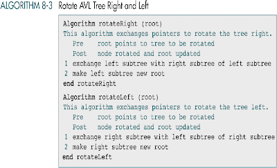
Rotate AVL Tree Right and Left:

AVL Tree delete:

Algorithms & Data Structures - AVL TREE

• A balance binary search tree.
• The best search time, that is O(log N) search times


• An AVL tree is defined to be a well-balanced binary search tree in which each of its nodes has the AVL property.
• The AVL property is that the heights of the left and right sub-trees of a node are either equal or if they differ only by 1

Keeping the Tree Balance

• the height of the right subtree and height of the left subtree for any node cannot differ by more than one.
• This process is usually done through rotation.

Diagram 1


• A single counter clockwise rotate will balance it.
• s_ right_rotate() - because it involves the right subtree.

Diagram 2


• A single counter clockwise rotate will balance it.
• s_ left_rotate() - because it involves the left subtree.

Diagram 3


• A double clockwise rotate will balance it.
• 1st - single clockwise rotation with the parent of the inserted node (this produces the tree in diagram 1)
• 2nd - single counter clockwise rotation on the root
• d_ right_rotate() - because it involves the right subtree.

Diagram 4


• A double clockwise rotate will balance it.
• 1st - single counter clockwise rotation with the parent of the inserted node (this produces the tree in diagram 2)
• 2nd - single clockwise rotation with the root.
• d_ left_rotate() - because it involves the left subtree.

Example:
Given these data: build an AVL tree.
12 , 10 , 3 , 23 , 11, 14 , 2 , 4 , 1
Click the picture below to see the answer! ^_^

Algorithms & Data Structures - Sorting 1 and Analysis

• Sort problem is obvious to all
• Several distinct algorithms to solve it
• Algorithms use different data structures
• Algorithm performance varies widely
• See Chapters 1, 2, and 7
• For now, skip ShellSort and QuickSort
• Bubble Sort
• Insertion Sort
• Merge Sort
• And analysis as we go…

BubbleSort
procedure BubbleSort( var A : InputArray; N : int);
var
j, P : integer;
begin
for P := N to 2 by -1 do begin
for j := 1 to P - 1 do begin
if A[ j ] > A[ j + 1 ] then
Swap( A[ j ], A[ j + 1 ] );
end; {for}
end; {for}
end;

Template BubbleSort class
template<class T> class CBubbleSort {
public:
void Sort(T *A, int N)
{
for(int P = N-1; P >= 1; P--)
{
for(int j = 0; j<＝P-1; j++) { if(A[j + 1] < t =" A[j">Utilizing it…

// Data …
vector<double> data;

// fill in the data…

// Instantiate the sort object…
CBubbleSort<double> sort;

sort.Sort(&data[0], data.size());

Running time for BubbleSort
How many times does c,d get executed?
for P := N to 2 by -1 do begin
for j := 1 to P - 1 do begin
if A[ j ] > A[ j + 1 ] then
Swap( A[ j ], A[ j + 1 ] );
end; {for}
end; {for}

Running time for BubbleSort
How many times does c,d get executed?

So, we could say:


Big-Oh notation
Definition: T(N)=O( f(N) ) if there are positive constants c and n0 such that T(N) <= cf(N) when N >= n0
Another notation:

Intuitively what does this mean?

Asymptotic Upper Bound


Example of Asymptotic Upper Bound




Is BubbleSort O(N2)?

Can we find a c and n0?:

Some rules to simplify things…

• Loops:
• Running time is body time times # iterations
• Nested loops:
• Analysis from the inside out…
• Statements:
• Assume time of 1 each
• Unless the statement is an algorithm
• So, we could say:

Usage


Exercise in Big O-notation


What’s the minimum time?


Omega notation







Asymptotic Lower Bound


What these tell us

O(f(N)) - Upper bound on running timg

Ω(g(N)) - Lower bound on running time

What about the “constants”?

• Algorithm 1: O(N), actual time is:
• T(N)=1,000,000N
• Algorithm 2: O(N2), actual time is:
• T(N)=10N2
• When is algorithm 2 faster?

Why do we care?

• After all, computers just keep getting faster, don’t they?
• Is today’s slow algorithm acceptable tomorrow?
• Algorithm 1: O(N2)
• Algorithm 2: O(N)
• If your computer is suddenly 10 times faster, can you handle 10 times as much data in the same time?

Faster Computer or Algorithm?
√ What happens when we buy a computer 10 times faster?


Constant running time


Theta Notation


Big O, Omega, Theta


In general:
O is used to denote the upper bound of the complexity
Ω is used to denote the lower bound of the complexity
Ø is used to denote the tight bound of the complexity

Example, the general sorting problem has the time complexity Ω(nlogn). Any sorting based on compare-interchange takes c.nlogn time for some constant c.

Sorting problem has a time complexity O(nlogn)
(since there is an algorithm which sorts in O(nlogn) time)

Aside: Can we make this faster in some cases?
procedure BubbleSort( var A : InputArray; N : int);
var
j, P : integer;
begin
for P := N to 2 by -1 do begin
for j := 1 to P - 1 do begin
if A[ j ] > A[ j + 1 ] then
Swap( A[ j ], A[ j + 1 ] );
end; {for}
end; {for}
end;

Insertion Sort
procedure InsertionSort( var A : InputArray; N : integer);
var j, P : integer; Tmp : InputType;
begin
for P := 2 to N do begin
j := P;
Tmp := A[ P ];

while j > 1 and Tmp < A[ j - 1 ] do begin
A[ j ] := A[ j - 1 ];
j := j - 1;
end; {while}
A[ j ] := Tmp;
end; {for}
end;

Worst case analysis

• N outer loops
• Each item moved maximum distance
• For item i, that would be i-1, right?

Best case analysis

• N outer loops
• Each is not moved at all
• For item i, 0 moves, which is constant time.

Worst-Case and Average-Case Analysis

• Worst-case analysis
• Big O, the upper bound, of the running time of any input of size N.
• Average-case analysis
• Some algorithms are fast in practice.
• The analysis is usually much harder.
• Need to assume that all input are equally likely.
• Sometimes, it is not obvious what is the average.

InsertionSort Average Case

On average, how much would you have to move a item to sort the list?

For item i, the minimum is 0 and the maximum is i-1. So, the average is i/2

Insertion Sort Average CaseMore formal solution

• For sorting, we assume randomly ordered data.
• Inversions:
• An inversion in an array of numbers is any ordered pair (i, j) having the property that
• i < j and A[i] > A[j]
• How many inversions in this list:
• 12, 17, 5, 7, 21, 1, 8
• How many are possible altogether?

Inversions
√ The maximum inversions for a list of size N is N(N-1)/2
√ Theorem: The average number of inversions in an array of N distinct numbers is N(N-1)/4

Average case for exchanging adjacent elements
√ When we exchange adjacent elements we remove exactly one inversion

• 12, 17, 5, 7, 21, 1, 8

√ We have to remove on average N(N-1)/4 inversions=Ω(N2)

Mergesort
procedure MergeSort( var A : InputArray; N : int);
Begin
MSort(A, 1, N)
end;

Procedure MSort(var A : InputArray; F, L : int);
var q: int;
Begin
if F < L then begin
q := (F + L) / 2
MSort(A, F, Q);
MSort(A, Q+1, L);

Merge(A, F, Q, L);
end;
End;



How long does merge take?

• One of the earliest sorting sorting algorithms, invented by John von Neumann in 1945.
• Mergesort is Divide-and-conquer Algorithm
• Given an instance of the problem to be solved, split this into several, smaller, sub-instances (of the same problem) independently solve each of the sub-instances and then combine the sub-instance solutions so as to yield a solution for the original instance.
• The problem is divided into smaller problems and solved recursively.
• Quicksort and heapsort are also such algorithms

Running Time

T(1)=O(1)

T(N)=T(N/2)+T(N/2)+O(N)

Mergesort

• O(n log n) worst-case running time
• Same ops done regardless of input order
• Mergesort is Divide-and-conquer Algorithm
• Copying to and from temporary array
• Extra memory requirement
• Extra work